This notebook is based on a worksheet by Radovan Omorjan.
We will solve the boundary value problem for the second order ordinary differential equation given in the form
y" + g1(x,y)*y' + g2(x,y)*y = g3(x)
with the boundary conditions
A*y(x=a) + B*y'(x=a) = C
A1*y(x=b) + B1*y'(x=b) = C1
y" - phi*y^n = 0
Boundary conditions
  y(x=0)= 0.1
  y(x=1)= 1
phi,n are given constants
Defining the function of the derivatives, we set y[1]=y, y[2]=y' therefore
  y[1]'=y[2]
  y[2]'=g3(x)-g2(x,y[1])*y[1]-g1(x,y[1])*y[2]
>function deriv(x,y) := [y[2],g3(x)-g2(x,y[1])*y[1]-g1(x,y[1])*y[2]]
The user has to define functions g1(x,y),g2(x,y),g3(x), f0(x) and the guess value for y'(0).
>function g1(x,y) := 0
>function g2(x,y) := -phi*y^n/y
>function g3(x) := 0
Defining the function in single variable which has zero values in the solution (see the given boundary conditions)
>function f0(ydguess) := lsoda("deriv",[0,1],[0.1,ydguess])[1,2]
We use this values.
>phi=4; n=1;
Let us try to values.
>f0(0), f0(1)
0.376219569124
2.18964977308
>res=secant("f0",0,2,y=1)
0.343978185375
Should be close to 1.
>f0(res)
1
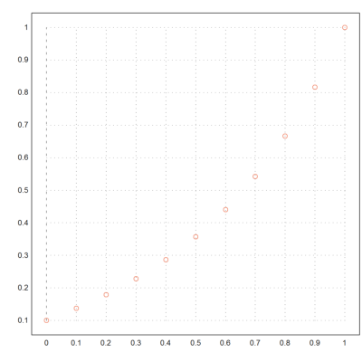
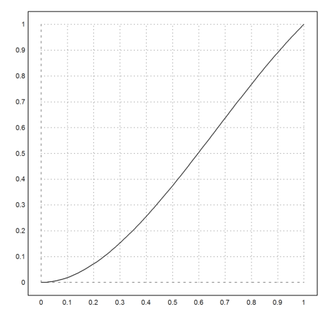
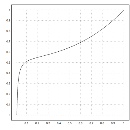
Plotting the result!
>t=0:0.1:1; y=lsoda("deriv",t,[0.1,res]); ...
 plot2d(t,y[1],color=10,points=1,style="o"); ...
 insimg(25,"");
This simple example of boundary value problem for second order ODE could also be solved in Maxima analytically.
>function g1(x,y) &= 0
0
>function g2(x,y) &= -phi*y^n/y
                                    n - 1
                             - phi y
>function g3(x) &= 0
0
>equ &= 'diff(y,x,2) + g1(x,y)*'diff(y,x) + g2(x,y)*y = g3(x)
                            2
                           d y        n
                           --- - phi y  = 0
                             2
                           dx
>res &= ode2(subst([n=1,phi=4],equ),y,x)
                               2 x        - 2 x
                      y = %k1 E    + %k2 E
>res1 &= rhs(bc2(res,x=0,y=1/10,x=1,y=1))
                     2       2 x     4       2   - 2 x
                (10 E  - 1) E      (E  - 10 E ) E
                ---------------- + -------------------
                       4                   4
                   10 E  - 10          10 E  - 10
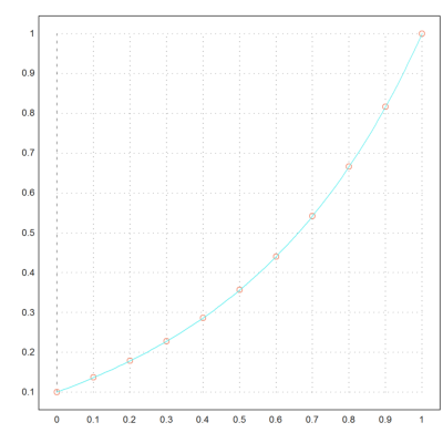
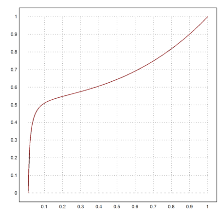
Plotting numerical (points) and analytical solutions (line)
>x=0:0.01:1; plot2d(x,res1(x),add=true,color=13); ...
 insimg(25,"");
We solve a very special case, where the derivative function has a singularity at the boundary.
  y'' = 2y'/x - 4y
  y(0)=0
  y(1)=1
>function f(x,y) := [ y[2], 2*y[2]/x-4*y[1] ]
The singularity is removed if y'(0)=0. So this function might have a nice solution. However, y(0)=0, and y'(0)=0 always yield the zero function for normal problems (e.g. Lipschitz continous f). Thus we expect problems.
In fact there is no proper way to shoot from 0 to 1. So we do a backward shooting.
Setup the shooting from x=1, y=1, back to 0, a function depending on y'(1).
>function g(der) := lsoda("f",[1,0],[1,der])[1,-1]
>g(1)
0.236949825926
Find a derivative y'(1)=der with y(0)=0.
>der1 = secant("g",2.5)
2.0884291999
Plot the correct solution.
>x=1:-0.01:0; y=lsoda("f",x,[1,der1]); plot2d(x,y[1]):
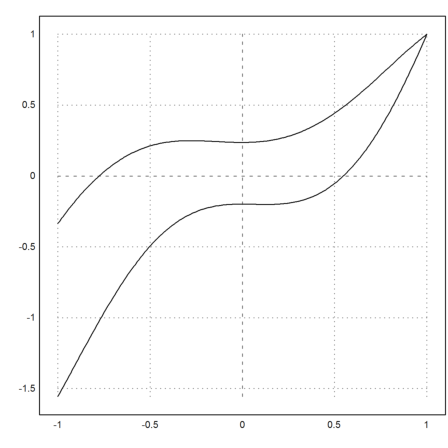
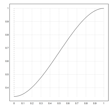
Plot two shootings. All of them are defined across x=0.
>x=1:-0.01:-1; y=lsoda("f",x,[1,3]); plot2d(x,y[1]); ...
 x=1:-0.01:-1; y=lsoda("f",x,[1,1]); plot2d(x,y[1],add=true); ...
 insimg;
Let us try a simpler example.
  y'' = 2*y'/x-4
  y(0) = 0
  y(1) = 1
>function f(x,y) := [ y[2], 2*y[2]/x-4 ]
>function g(der) := lsoda("f",[1,0],[1,der])[1,-1]
>der1 = secant("g",2.5)
1.00000000001
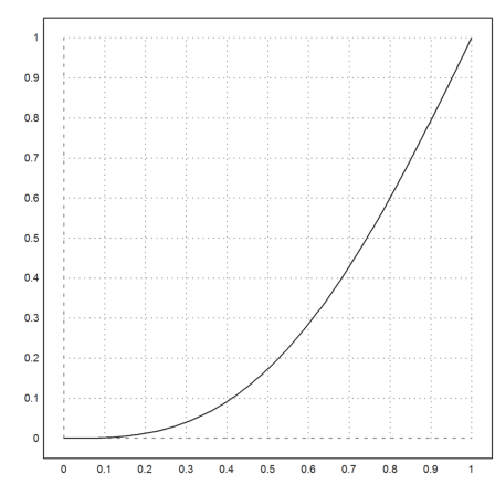
Plot the correct solution.
>x=1:-0.01:0; y=lsoda("f",x,[1,der1]); plot2d(x,y[1]):
We can solve this with Maxima.
>sol &= ode2('diff(y,x,2)=2*'diff(y,x)/x-4,y,x)
                                3      2   %k1
                       y = %k2 x  + 2 x  - ---
                                            3
>function y(x,%k1,%k2) &= rhs(sol)
                              3      2   %k1
                         %k2 x  + 2 x  - ---
                                          3
>&diff(y(x,a,b),x,2) = expand(-2*diff(y(x,a,b),x)/x-4)
6 b x + 4 = - 6 b x - 12
>&solve(y(1,a,b)=1,[a,b]);  ...
   function y1(x,c) &= y(x,a,b) with %[1] with %rnum_list[1]=c
                          3      2   - 3 c - 3
                       c x  + 2 x  + ---------
                                         3
>&expand(y1(1,c))
1
>&diff(y1(x,c),x) with x=1
3 c + 4
>plot2d("y1(x,-4/3)",0,1):
The following problem does not have a solution.
  y'' = -2*y'/x-4
  y(0) = 0
  y(1) = 1
From the general solution you see that the boundary conditions cannot hold.
>sol &= ode2('diff(y,x,2)=-2*'diff(y,x)/x-4,y,x)
                                 2
                              2 x    %k2
                        y = - ---- + --- + %k1
                               3      x
The following example has the solution y(x)=sqrt(x)
  y'' = -1/2*y'/x
  y(0)=0
  y(1)=1
>&sqrt(x); &diff(%,x,2) + 1/2 *diff(%,x)/x
0
The shooting method is hard to do, since lsoda will fail, if x is too close to 0.
>function f(x,y) := [ y[2], -1/2*y[2]/x ]
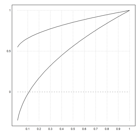
Let us try two shootings from x=1, but only to 0.01
>x=1:-0.01:0.01; ...
 y1=lsoda("f",x,[1,1/4])[1]; ...
 y2=lsoda("f",x,[1,3/4])[1]; ...
 plot2d(x,y1_y2):
>function h(der) := lsoda("f",[1,1e-4],[1,der])[1,2];
That is almost the best we can do. The correct answer is 0.5.
>der0:=bisect("h",1/4,3/4)
0.505050504939
The problem changes again, if we add another term to the solution.
>function f(x,y) := [ y[2], -2*y[2]/x + 4*y[1] ]
Let us try some shooting.
>x=1:-0.01:0.01; ...
 y1=lsoda("f",x,[1,1.2])[1]; ...
 y2=lsoda("f",x,[1,1])[1]; ...
 plot2d(x,y1_y2):
>function h(der) := lsoda("f",[1,0.01],[1,der])[1,2];
>der0:=bisect("h",1,1.2)
1.07773431527
The solution with y(0.01)=0 looks like this.
>y=lsoda("f",x,[1,der0])[1]; ...
 plot2d(x,y):
There is a nice solution to this equation.
>function f(x,a,b) &= a*exp(-2*x)/x + b*exp(2*x)/x
                             2 x      - 2 x
                          b E      a E
                          ------ + --------
                            x         x
We can solve it for y(1)=1, y(s)=0.
>sol &= solve([f(1,a,b)=1,f(s,a,b)=0],[a,b])
                           4 s + 2           2
                          E                 E
                  [[a = - ---------, b = ---------]]
                           4    4 s       4    4 s
                          E  - E         E  - E
And make the solution a function.
>function fsol(x,s) &= factor(f(x,a,b) with sol[1])
                2 - 2 x   x    s    x    s    2 x    2 s
               E        (E  - E ) (E  + E ) (E    + E   )
             - ------------------------------------------
                      s        s        2 s    2
                    (E  - E) (E  + E) (E    + E ) x
Let us check.
>&ratsimp(diff(fsol(x,s),x,2)+2*diff(fsol(x,s),x)/x-4*fsol(x,s))
0
Add the solution to the plot.
>plot2d("fsol(x,0.01)",color=red,add=true):
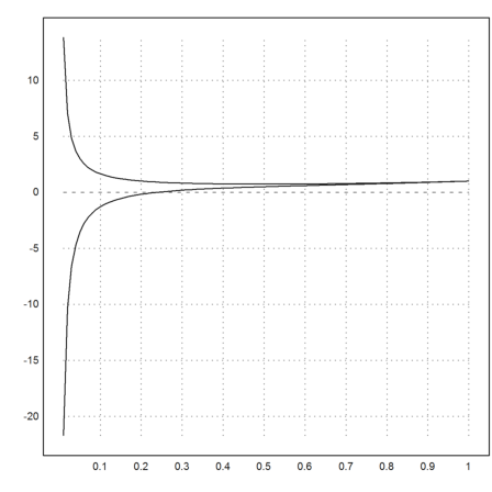
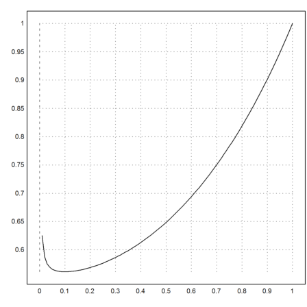
The limit for s->0 looks quite different.
>plot2d("fsol(x,0)",0,1):
Here, we have the function.
>&ratsimp(fsol(x,0))
                         - 2 x   4 x + 2    2
                        E      (E        - E )
                        ----------------------
                                4
                              (E  - 1) x
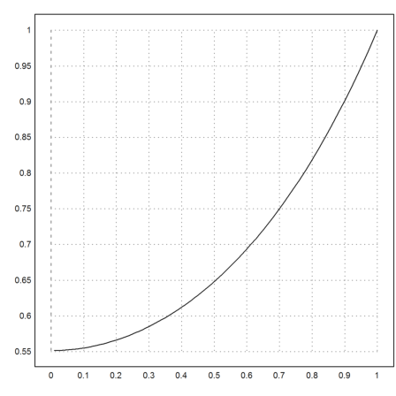
We can also solve it for y'(s)=0. Let us define the function for the derivative.
>function fd(x,a,b) &= diff(f(x,a,b),x)
                   2 x      2 x        - 2 x      - 2 x
              2 b E      b E      2 a E        a E
              -------- - ------ - ---------- - --------
                 x          2         x            2
                           x                      x
And solve it.
>sol &= solve([f(1,a,b)=1,fd(s,a,b)=0],[a,b])
                              4 s + 2
                   (2 s - 1) E
        [[a = -----------------------------,
                         4 s    4
              (2 s - 1) E    + E  (2 s + 1)
                                                2
                                               E  (2 s + 1)
                                   b = -----------------------------]]
                                                  4 s    4
                                       (2 s - 1) E    + E  (2 s + 1)
Make the solution a function.
>function fsol(x,s) &= factor(f(x,a,b) with sol[1])
              2 - 2 x       4 x    4 x        4 s    4 s
             E        (2 s E    + E    + 2 s E    - E   )
             --------------------------------------------
                        4 s    4 s      4      4
                  (2 s E    - E    + 2 E  s + E ) x
>plot2d("fsol(x,0.1)",0,1):
The solution for y'(0)=0 happens to be the same as y(0)=0.
>&fsol(x,0)
                          2 - 2 x   4 x
                         E        (E    - 1)
                         -------------------
                               4
                             (E  - 1) x